
Table of Contents:-
- Meaning of Portfolio Evaluation
- Portfolio Evaluation Methods
- Sharpe’s Measure/Sharpe’s Ratio
- Treynor’s Measure/Treynor’s Ratio
- Jensen Measure/Jensen Ratio
- Modigliani & Modigliani Measure (M² Measure)
Meaning of Portfolio Evaluation
Portfolio evaluation involves the evaluation of the performance of the portfolio. It is the fundamental process that involves comparing the returns generated by a portfolio with the return earned on one or more other portfolios or a benchmark portfolio. Portfolio evaluation consists of two major functions:
- Performance measurement and
- Performance evaluation.
Performance measurement is an accounting function which measures the return earned on a portion during the holding period or investment period.
Performance evaluation, on the other hand, determines whether the performance was superior or inferior and whether the performance was a result of skill or luck.
When assessing a portfolio’s performance, the return earned on the portfolio must be essentially evaluated concerning the risk associated with that portfolio. One approach would be to group portfolios into equivalent risk classes and then compare the returns of portfolios within each risk category. An alternative approach would be to specifically adjust the return for the riskiness of the portfolio by developing risk-adjusted return measures and using these for evaluating portfolios across differing risk levels.
Portfolio Evaluation Methods
Portfolio evaluation methods are as follows:
- Sharpe ratio
- Treynor ratio
- Jensen’s Ratio
- Modigliani and Modigliani
Sharpe’s Measure/Sharpe’s Ratio
Sharpe’s measure is also known as the ‘Reward to Variability’ Ratio. The returns from a portfolio are firstly adjusted for risk-free return. These excess returns, which serve as a reward for investing in risky assets are then evaluated in terms of the return per unit of risk.
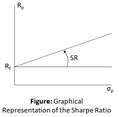 The image above represents Sharpe’s ratio:
Sharpe’s Ratio Formula:
$$\mathrm{Sharpe}’\mathrm s\;\mathrm{Ratio}\;(\mathrm{SR})\;=\;\left[\frac{{\mathrm R}_{\mathrm P}-{\mathrm R}_{\mathrm F}}{{\mathrm\sigma}_{\mathrm P}}\right]$$
Where,
Rp = Realized Return on a portfolio during a holding period
RF = Risk-free rate of Return
σP = Standard deviation of the Portfolio
Example: Let us consider two portfolios and calculate the Sharpe ratio for each.
| Portfolio | Return (RP) | Risk-Free (RF) | Excess return (RP – PF ) |
Portfolio risk (SD) |
| A | 32 | 10 | 22 | 12 |
| B | 20 | 11 | 9 | 7 |
Solution: $$\mathrm{Sharpe}’\mathrm s\;\mathrm{Ratio}\;:\;\mathrm{Portfolio}\;\mathrm A\;\;=\;\left[\frac{32-10}{12}\right]\;=\;1.8333\\\mathrm{Portfolio}\;\mathrm B\;=\;\left[\frac{20\;-\;11}7\right]\;=\;1.285$$
In the case of Portfolio A the reward per unit of risk is relatively higher. Hence it indicates that its performance is good.
Example: Calculate the Sharpe Ratio for the four different portfolios based on the data given below.
| Portfolio | Expected Rate of Return |
SD of Returns from Portfolios |
| P | 15% | 9.00 |
| Q | 10% | 3.00 |
| R | 14% | 7.50 |
| S | 11% | 6.00 |
The expected rate of return on the market portfolio is 8.50% with an SD of 3. The RF(risk-free rate) is 5%. Which portfolio has performed the best?
| Portfolio |
Sharpe Ratio |
| P | (15 – 5)/6.00 = 1.000 |
| Q | (10 – 5)/ 3.00 = 1.6667 |
| R | ( 14 – 5)/ 7.50 = 1.2000 |
| S | ( 11 – 5)/6.00 = 1.000 |
Therefore, Portfolio R is the strongest performer.
Treynor’s Measure/Treynor’s Ratio
Treynor’s measure is also known as the ‘Reward to Volatility ratio’. Treynor considers portfolio beta as a measure of risk Portfolio beta is the average beta of individual assets in the given Portfolio. This beta designates the market risk of the given portfolio.
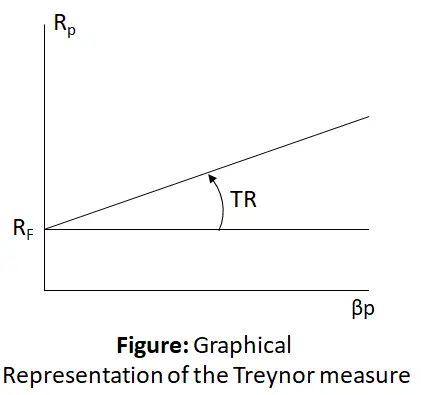 The Treynor’s measure is shown in the above image.
$$\mathrm{Treynor}’\mathrm s\;\mathrm{Measure}\;(\mathrm{TR})\;=\;\left[\frac{{\mathrm R}_{\mathrm P}\;-\;{\mathrm R}_{\mathrm F}}{{\mathrm\beta}_{\mathrm P}}\right]$$
where,
RP = Realized Return on a Portfolio
RF = Risk-free Rate of Return
βP = Portfolio
Example: Assume that you are an administrator of a pension fund, such as ICICI Prudential Life Time Pension Funds and you have to decide whether to renew your contracts with your three money managers. You must measure how they have performed to make an informed decision.
Consider the following performance results for each individual:
- Market return of 14%,
- Risk-free rate of 8%, and
- Beta of 1.
|
Investment Manager |
Average Annual Rate of Return |
Beta |
| W | 0.14 | 1.00 |
| X | 0.18 | 1.20 |
| Y | 0.16 | 1.05 |
| Z | 0.12 | 0.90 |
Solution: The T values for each investment manager can be calculated as :
$${\mathrm T}_{\mathrm W\;\;}=\;\left[\frac{0.14\;-\;0.08}{1.00}\right]\;=\;0.06\\\\{\mathrm T}_{\mathrm X}\;=\;\left[\frac{0.18\;-\;0.08}{1.20}\right]\;=\;0.083\\\\{\mathrm T}_{\mathrm Y}\;=\;\left[\frac{0.16\;-\;0.08}{1.05}\right]\;\;=\;0.076\\\\{\mathrm T}_{\mathrm Z\;}\;=\;\left[\frac{0.12\;-\;0.8}{0.90}\right]\;=\;0.044\\\\$$
These results show that Z did not outperform the market. X had the strongest performance and both Y and X surpassed market expectations.
Example: Calculate the Treynor Ratio based on the performance of four portfolio managers over five years. Use the data given below
- The risk-free rate (RF) is 10% and
- The market return (RM) is 16%.
| Portfolio Manager | Average Return (%) | Beta |
| P | 15 | 0.90 |
| Q | 17 | 1.25 |
| R | 17 | 1.05 |
| S | 14 | 0.80 |
Choose the portfolio manager that has performed best.
Solution:
| Portfolio Manager | Treynor Ratio | Treynor Ratio |
| P | $$\frac{(15\;-\;10)}{0.90}=\;5.555$$ | 5.555 |
| Q | $$\frac{(17\;-\;10)}{1.25}=\;5.600$$ | 5.600 |
| R | $$\frac{(17\;-\;10)}{1.05}=\;6.666$$ | 6.666 |
| S | $$\frac{(14\;-\;10)}{0.80}=\;5.000$$ | 5.000 |
Therefore, Q is the strongest performer among all.
Jensen Measure/Jensen Ratio
The Treynor and Sharpe Indexes provide measures for evaluating the relative performances of various portfolios, taking into account the level of risk involved. Jensen attempts to construct a measure of absolute performance on a risk-adjusted basis Le, a definite standard against which performances of various funds can be measured.
This standard is based on the measurement of the “portfolio manager’s predictive ability i.e., his ability to earn returns through successful prediction of security prices which are higher than those which we would expect given the level of riskiness of his portfolio”.
A simplified version of his basic model is given as follows:
$${\overline{\mathrm R}}_{\;\mathrm{jt}}\;-\;{\mathrm R}_{\mathrm{ft}}\;=\;{\mathrm\alpha}_{\mathrm j}\;+\;{\mathrm\beta}_{\mathrm j}\;({\overline{\mathrm R}}_{\mathrm{mt}}\;-\;{\mathrm R}_{\mathrm{ft}})\\$$
Where,
- $${\overline{\mathrm R}}_{\;\mathrm{jt}}\;=\;\mathrm{Average}\;\mathrm{return}\;\mathrm{on}\;\mathrm{portfolio}\;\mathrm j\;\mathrm{for}\;\mathrm{period}\;\mathrm t,$$
- $${\mathrm R}_{\mathrm{ft}}\;=\;\mathrm{Risk}-\mathrm{free}\;\mathrm{rate}\;\mathrm{of}\;\mathrm{interest}\;\mathrm{for}\;\mathrm{period}\;\mathrm t,$$
- $${\mathrm\beta}_{\mathrm j}\;=\;\mathrm{Measure}\;\mathrm{of}\;\mathrm{systematic}\;\mathrm{risk},$$
- $${\overline{\mathrm R}}_{\mathrm{mt}}\;=\mathrm{The}\;\mathrm{average}\;\mathrm{return}\;\mathrm{of}\;\mathrm a\;\mathrm{market}\;\mathrm{portfolio}\;\mathrm{for}\;\mathrm a\;\mathrm{period}\;\mathrm t.\;$$
- $$\alpha_j\;=\;Measures\;forecasting\;ability$$
An implication of forms of the Sharpe and Treynor models is that the intercept of the line is at the origin. In the Jensen model, the intercept can be at any point, including the origin.
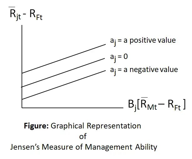 For example, in the above image, the upper line represents a case of superior management performance. In fact, o, a positive value represents the average superior extra return accruing to that particular portfolio because of superior management talent.
The line αj = 0 indicates neutral performance by management; i.e., management has done as well as an unmanaged market portfolio or a large, randomly selected portfolio managed with a naive buy-and-hold strategy.
The lower line, αj = a negative value, indicates inferior management performance because management did not do as well as an unmanaged portfolio of equal systematic risk. This situation could arise in part because portfolio returns were not sufficient to offset the expenses incurred in the selection and management process.
The intercept may be interpreted in this fashion by examining the above formula. This occurs because if the portfolio manager is performing in a superior fashion, his intercept will have a positive value. After all, it will indicate that his portfolio is consistently over-performing the overall market. This would happen if the manager either had a superior ability to select undervalued securities or had a superior ability to recognize turning points in the market.
On the other hand, a negative intercept would indicate that the manager consistently underperformed the overall market. In other words, the risk-adjusted returns of his portfolio were consistently lower than the risk-adjusted returns of the market during the same period.
Example: Calculate the Actual Return and Risk
| Funds | Rft | Rjt | Rmt | Beta |
| Fund X | 5 | 12 | 15 | 0.5 |
| Fund Y | 5 | 20 | 15 | 1.0 |
| Fund Z | 5 | 14 | 15 | 1.10 |
Solution: From equation 1 return on the portfolio is:
-
$${\overline{\mathrm R}}_{\;\mathrm{jt}}\;-\;{\mathrm R}_{\mathrm{ft}}\;=\;{\mathrm\alpha}_{\mathrm j}\;+\;{\mathrm\beta}_{\mathrm j}\;({\overline{\mathrm R}}_{\mathrm{mt}}\;-\;{\mathrm R}_{\mathrm{ft}})\\$$
- $$\alpha\;=r_p\;-\;r_{jt}$$
Fund X:
Rjt = 5 + 0.5 (15 – 5) = 10
α = 12-10 = 2% (Excess Positive Return)
Fund Y:
Rjt = 5 + 1.5 (15 – 5) = 15
α = 20-15 = 5% (Excess Positive Return)
Fund Z:
Rjt = 5 + 1.10 (15 – 5) = 16
α = 14-16 = -20% (Negative Return)
Example: Calculate Jenson’s Alpha based on the results of four portfolio managers for 5 years. Use the data given below to choose the manager with the best performance.
- The risk-free rate (RF) is 10% and
- The market return (RM) is 16%.
| Portfolio Manager | Average Return (%) | Beta |
| P | 15 | 0.90 |
| Q | 17 | 1.25 |
| R | 17 | 1.05 |
| S | 14 | 0.80 |
Solution: Q is the best performer.
| Portfolio Manager | Treynor Ratio | Treynor Ratio |
| P | 15 – [10 + 0.80(16 – 10)] = -0.40 | -0.40 |
| Q | 15 – [10 + 0.80(16 – 10)] = -0.50 | -0.50 |
| R | 15 – [10 + 0.80(16 – 10)] = 0.70 | 0.70 |
| S | 15 – [10 + 0.80(16 – 10)] = -0.80 | -0.80 |
Modigliani & Modigliani Measure (M² Measure)
Modigliani Modigliani measure, which is referred to as M’ provides a risk-adjusted measure of performance that has an economically meaningful interpretation.
The M2 is given by M2 = rp* – rm
where, M2 Modigliani – Modigliani measure,
rp* = return on the adjusted portfolio,
rm = return on the market portfolio.
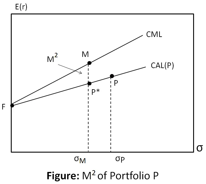 A graphical representation of the M2 measure appears in the above image. It moves down the capital allocation line corresponding to portfolio P (by mixing P with T-bills) until it reduces the standard deviation of the adjusted portfolio to match that of the market index. The M³ measure is then the vertical distance (ie, the difference in expected returns) between portfolios P* and M.
The above image shows that P will have a negative M2 measure when its capital allocation line is less steep than the capital market line, i.e., when its Sharpe ratio is lower than that of the market index.
Example: Calculate the following performance measures for portfolio P and the market M. The T-bill rate during the period is 6%. By which measures did the P portfolio outperform the market?
Use the following data for a particular sample period.
| Portfolio P | Market M | |
| Average return | 35% | 28% |
| Beta | 1.20% | 1.00% |
| Standard Deviation | 42% | 30% |
| Tracking error (non-systematic risk), σ(e) | 18% | 0 |
Solution: P has a standard deviation of 42% versus a market standard deviation of 30%.
Therefore, the adjusted portfolio P would be formed by mixing bills and portfolio P with weights 30/42 = 0.714 in P and 1 – 0.714 = 0.286 in bills.
The return on this portfolio would be (0. 286 × 6%) + (0.714 × 35%) = 26.7%, which is 1.3% less than the market return.
Thus, portfolio P has an M2 measure of -1.3 %.